Example ML Flow

Introduction

We’ll consider a typical (but simplified) machine learning flow.

(The code for this example is available in the Bionic repo at example/ml_workflow.py. Run pip install bionic[examples] to ensure you have the required dependencies.)

'''
A toy ML workflow intended to demonstrate basic Bionic features.  Trains a
logistic regression model on the UCI ML Breast Cancer Wisconsin (Diagnostic)
dataset.
'''

import re

from sklearn import datasets, model_selection, linear_model, metrics
import pandas as pd

import bionic as bn

# Initialize our builder.
builder = bn.FlowBuilder('ml_workflow')

# Define some basic parameters.
builder.assign('random_seed', 0)
builder.assign('test_split_fraction', 0.3)
builder.assign('hyperparams_dict', {'C': 1})
builder.assign('feature_inclusion_regex', '.*')


# Load the raw data.
@builder
def raw_frame():
    dataset = datasets.load_breast_cancer()
    df = pd.DataFrame(
        data=dataset.data,
        columns=dataset.feature_names,
    )
    df['target'] = dataset.target
    return df


# Select a subset of the columns to use as features.
@builder
def features_frame(raw_frame, feature_inclusion_regex):
    included_feature_cols = [
        col for col in raw_frame.columns.drop('target')
        if re.match(feature_inclusion_regex, col)
    ]
    return raw_frame[included_feature_cols + ['target']]


# Split the data into train and test sets.
@builder
# The `@outputs` decorator tells Bionic to define two new entities from this
# function (which returns a tuple of two values).
@bn.outputs('train_frame', 'test_frame')
def split_raw_frame(features_frame, test_split_fraction, random_seed):
    return model_selection.train_test_split(
        features_frame,
        test_size=test_split_fraction,
        random_state=random_seed,
    )


# Fit a logistic regression model on the training data.
@builder
def model(train_frame, random_seed, hyperparams_dict):
    m = linear_model.LogisticRegression(
        solver='liblinear', random_state=random_seed,
        **hyperparams_dict)
    m.fit(train_frame.drop('target', axis=1), train_frame['target'])
    return m


# Evaluate the model's precision and recall over a range of threshold values.
@builder
def precision_recall_frame(model, test_frame):
    predictions = model.predict_proba(test_frame.drop('target', axis=1))[:, 1]
    precisions, recalls, thresholds = metrics.precision_recall_curve(
        test_frame['target'], predictions)

    df = pd.DataFrame()
    df['threshold'] = [0] + list(thresholds) + [1]
    df['precision'] = list(precisions) + [1]
    df['recall'] = list(recalls) + [0]

    return df


# Plot the precision against the recall.
@builder
# The `@pyplot` decorator makes the Matplotlib plotting context available to
# our function, then translates our plot into an image object.
@bn.pyplot('plt')
# The `@gather` decorator collects the values of of "hyperparams_dict" and
# "precision_recall_frame" into a single dataframe named "gathered_frame".
# This might not seem very interesting since "gathered_frame" only has one row,
# but it will become useful once we introduce multiplicity.
@bn.gather(
    over='hyperparams_dict',
    also='precision_recall_frame',
    into='gathered_frame')
def all_hyperparams_pr_plot(gathered_frame, plt):
    _, ax = plt.subplots(figsize=(4, 3))
    for row in gathered_frame.itertuples():
        label = ', '.join(
            '%s=%s' % key_value
            for key_value in row.hyperparams_dict.items()
        )
        row.precision_recall_frame.plot(
            x='recall', y='precision', label=label, ax=ax)
    ax.set_xlabel('Recall')
    ax.set_ylabel('Precision')


# Assemble our flow object.
flow = builder.build()

# Compute and print the precision-recall dataframe.
if __name__ == '__main__':
    bn.util.init_basic_logging()

    import argparse
    parser = argparse.ArgumentParser(
        description='Runs a simple ML workflow example')
    parser.add_argument(
        '--bucket', '-b', help='Name of GCS bucket to cache in')

    args = parser.parse_args()
    if args.bucket is not None:
        flow = flow\
            .setting('core__persistent_cache__gcs__bucket_name', args.bucket)\
            .setting('core__persistent_cache__gcs__enabled', True)

    with pd.option_context("display.max_rows", 10):
        print(flow.get('precision_recall_frame'))

Let’s start by importing the flow into a notebook and visualizing it.

from example.ml_workflow import flow

flow.render_dag()

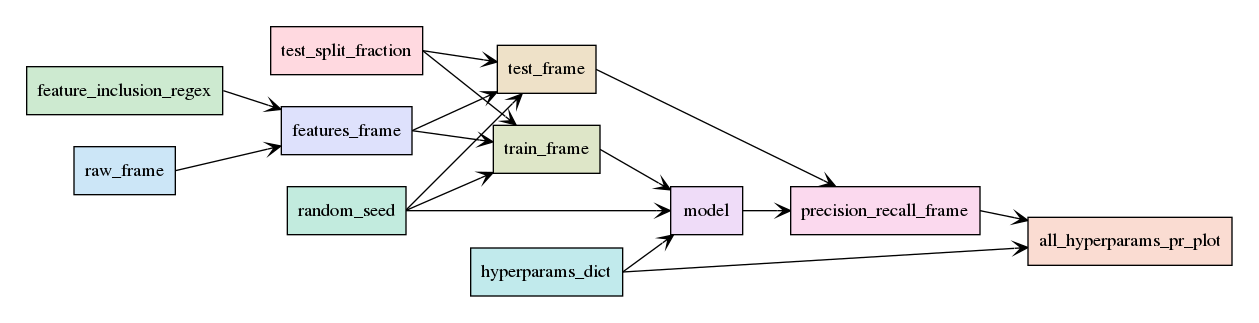
This is still a toy example, but it demonstrates a classic supervised machine learning flow for binary classification:

• Load data (raw_frame)

• Clean it (features_frame)

• Split into training and test sets (train_frame and test_frame)

• Fit a model on the training data (model)

• Evaluate the model on the test data (precision_recall_frame)

• Visualize the model’s performance (all_hyperparams_pr_plot)

As in the previous example, we can access any of the entity values. However, this time we’ll enable logging so we can see every entity that Bionic computes.

import logging; logging.basicConfig(level='INFO', format='%(message)s')

flow.get.train_frame().head()

Accessed    random_seed(random_seed=0) from definition
Accessed    test_split_fraction(test_split_fraction=0.3) from definition
Accessed    feature_inclusion_regex(feature_inclusion_regex=_.._12aca9f6a2) from definition
Computing   raw_frame() ...
Computed    raw_frame()
Computing   features_frame(feature_inclusion_regex=_.._12aca9f6a2) ...
Computed    features_frame(feature_inclusion_regex=_.._12aca9f6a2)
Computing   train_frame(feature_inclusion_regex=_.._12aca9f6a2, test_split_fraction=0.3, random_seed=0) ...
Computing   test_frame(feature_inclusion_regex=_.._12aca9f6a2, test_split_fraction=0.3, random_seed=0) ...
Computed    train_frame(feature_inclusion_regex=_.._12aca9f6a2, test_split_fraction=0.3, random_seed=0)
Computed    test_frame(feature_inclusion_regex=_.._12aca9f6a2, test_split_fraction=0.3, random_seed=0)

	mean radius	mean texture	mean perimeter	mean area	mean smoothness	mean compactness	mean concavity	mean concave points	mean symmetry	mean fractal dimension	...	worst texture	worst perimeter	worst area	worst smoothness	worst compactness	worst concavity	worst concave points	worst symmetry	worst fractal dimension	target
478	11.490	14.59	73.99	404.9	0.10460	0.08228	0.05308	0.01969	0.1779	0.06574	...	21.90	82.04	467.6	0.1352	0.2010	0.25960	0.07431	0.2941	0.09180	1
303	10.490	18.61	66.86	334.3	0.10680	0.06678	0.02297	0.01780	0.1482	0.06600	...	24.54	70.76	375.4	0.1413	0.1044	0.08423	0.06528	0.2213	0.07842	1
155	12.250	17.94	78.27	460.3	0.08654	0.06679	0.03885	0.02331	0.1970	0.06228	...	25.22	86.60	564.2	0.1217	0.1788	0.19430	0.08211	0.3113	0.08132	1
186	18.310	18.58	118.60	1041.0	0.08588	0.08468	0.08169	0.05814	0.1621	0.05425	...	26.36	139.20	1410.0	0.1234	0.2445	0.35380	0.15710	0.3206	0.06938	0
101	6.981	13.43	43.79	143.5	0.11700	0.07568	0.00000	0.00000	0.1930	0.07818	...	19.54	50.41	185.2	0.1584	0.1202	0.00000	0.00000	0.2932	0.09382	1

5 rows × 31 columns

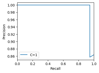
flow.get.all_hyperparams_pr_plot()

Accessed    train_frame(feature_inclusion_regex=_.._12aca9f6a2, test_split_fraction=0.3, random_seed=0) from in-memory cache
Accessed    test_frame(feature_inclusion_regex=_.._12aca9f6a2, test_split_fraction=0.3, random_seed=0) from in-memory cache
Accessed    hyperparams_dict(hyperparams_dict=70c34f2de8) from definition
Computing   model(feature_inclusion_regex=_.._12aca9f6a2, test_split_fraction=0.3, random_seed=0, hyperparams_dict=70c34f2de8) ...
Computed    model(feature_inclusion_regex=_.._12aca9f6a2, test_split_fraction=0.3, random_seed=0, hyperparams_dict=70c34f2de8)
Computing   precision_recall_frame(feature_inclusion_regex=_.._12aca9f6a2, test_split_fraction=0.3, random_seed=0, hyperparams_dict=70c34f2de8) ...
Computed    precision_recall_frame(feature_inclusion_regex=_.._12aca9f6a2, test_split_fraction=0.3, random_seed=0, hyperparams_dict=70c34f2de8)
Computing   all_hyperparams_pr_plot(feature_inclusion_regex=_.._12aca9f6a2, test_split_fraction=0.3, random_seed=0) ...
Computed    all_hyperparams_pr_plot(feature_inclusion_regex=_.._12aca9f6a2, test_split_fraction=0.3, random_seed=0)
Accessed    random_seed(random_seed=0) from in-memory cache

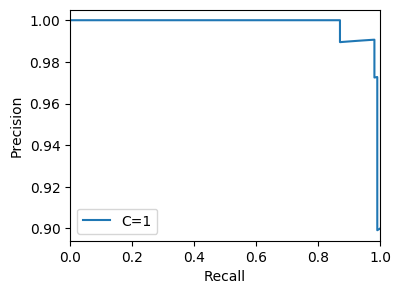
Note that in the logs, each entity is computed exactly once – every value is cached both in memory and on disk to avoid redundant computation.

Changing Inputs

Now that we have our flow, we might want to experiment with different parameter settings. For example, we can try changing our regularization hyperparameter C:

flow.setting('hyperparams_dict', {'C': 10}).get.all_hyperparams_pr_plot()

Accessed    hyperparams_dict(hyperparams_dict=ee67dd46dd) from definition
Loaded      train_frame(feature_inclusion_regex=_.._12aca9f6a2, test_split_fraction=0.3, random_seed=0) from disk cache
Loaded      test_frame(feature_inclusion_regex=_.._12aca9f6a2, test_split_fraction=0.3, random_seed=0) from disk cache
Accessed    random_seed(random_seed=0) from definition
Computing   model(feature_inclusion_regex=_.._12aca9f6a2, test_split_fraction=0.3, random_seed=0, hyperparams_dict=ee67dd46dd) ...
Computed    model(feature_inclusion_regex=_.._12aca9f6a2, test_split_fraction=0.3, random_seed=0, hyperparams_dict=ee67dd46dd)
Computing   precision_recall_frame(feature_inclusion_regex=_.._12aca9f6a2, test_split_fraction=0.3, random_seed=0, hyperparams_dict=ee67dd46dd) ...
Computed    precision_recall_frame(feature_inclusion_regex=_.._12aca9f6a2, test_split_fraction=0.3, random_seed=0, hyperparams_dict=ee67dd46dd)
Computing   all_hyperparams_pr_plot(feature_inclusion_regex=_.._12aca9f6a2, test_split_fraction=0.3, random_seed=0) ...
Computed    all_hyperparams_pr_plot(feature_inclusion_regex=_.._12aca9f6a2, test_split_fraction=0.3, random_seed=0)

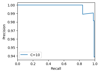
Bionic re-runs the flow with the changed parameter, generating a new plot.

Since we’ve created a new copy of our flow, Bionic doesn’t try to reuse its in-memory cache. However, we can see it that it only recomputed those entities whose values changed – the others were loaded from disk.

Similarly, we can try training our model on a subset of the available features:

flow.setting('feature_inclusion_regex', 'mean.*').get.all_hyperparams_pr_plot()

Accessed    random_seed(random_seed=0) from definition
Accessed    test_split_fraction(test_split_fraction=0.3) from definition
Accessed    feature_inclusion_regex(feature_inclusion_regex=mean.._a0ed126bd6) from definition
Loaded      raw_frame() from disk cache
Computing   features_frame(feature_inclusion_regex=mean.._a0ed126bd6) ...
Computed    features_frame(feature_inclusion_regex=mean.._a0ed126bd6)
Computing   train_frame(feature_inclusion_regex=mean.._a0ed126bd6, test_split_fraction=0.3, random_seed=0) ...
Computing   test_frame(feature_inclusion_regex=mean.._a0ed126bd6, test_split_fraction=0.3, random_seed=0) ...
Computed    train_frame(feature_inclusion_regex=mean.._a0ed126bd6, test_split_fraction=0.3, random_seed=0)
Computed    test_frame(feature_inclusion_regex=mean.._a0ed126bd6, test_split_fraction=0.3, random_seed=0)
Accessed    hyperparams_dict(hyperparams_dict=70c34f2de8) from definition
Computing   model(feature_inclusion_regex=mean.._a0ed126bd6, test_split_fraction=0.3, random_seed=0, hyperparams_dict=70c34f2de8) ...
Computed    model(feature_inclusion_regex=mean.._a0ed126bd6, test_split_fraction=0.3, random_seed=0, hyperparams_dict=70c34f2de8)
Computing   precision_recall_frame(feature_inclusion_regex=mean.._a0ed126bd6, test_split_fraction=0.3, random_seed=0, hyperparams_dict=70c34f2de8) ...
Computed    precision_recall_frame(feature_inclusion_regex=mean.._a0ed126bd6, test_split_fraction=0.3, random_seed=0, hyperparams_dict=70c34f2de8)
Computing   all_hyperparams_pr_plot(feature_inclusion_regex=mean.._a0ed126bd6, test_split_fraction=0.3, random_seed=0) ...
Computed    all_hyperparams_pr_plot(feature_inclusion_regex=mean.._a0ed126bd6, test_split_fraction=0.3, random_seed=0)

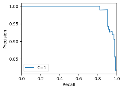
Naturally, reducing the number of features makes the model perform worse.

We can also apply this flow to a completely different dataset, such as the UCI ML Wine dataset. (This is actually a multiclass dataset, but to match the original example we’ll use binary labels.)

from sklearn import datasets
import pandas as pd

wine_data = datasets.load_wine()
wine_frame = pd.DataFrame(
    data=wine_data['data'],
    columns=wine_data['feature_names'])
wine_frame['target'] = (wine_data['target'] == 0)

wine_flow = flow.setting('raw_frame', wine_frame)
wine_flow.get.all_hyperparams_pr_plot()

Accessed    random_seed(random_seed=0) from definition
Accessed    test_split_fraction(test_split_fraction=0.3) from definition
Accessed    feature_inclusion_regex(feature_inclusion_regex=_.._12aca9f6a2) from definition
Accessed    raw_frame(raw_frame=70f5e80c40) from definition
Computing   features_frame(raw_frame=70f5e80c40, feature_inclusion_regex=_.._12aca9f6a2) ...
Computed    features_frame(raw_frame=70f5e80c40, feature_inclusion_regex=_.._12aca9f6a2)
Computing   train_frame(raw_frame=70f5e80c40, feature_inclusion_regex=_.._12aca9f6a2, test_split_fraction=0.3, random_seed=0) ...
Computing   test_frame(raw_frame=70f5e80c40, feature_inclusion_regex=_.._12aca9f6a2, test_split_fraction=0.3, random_seed=0) ...
Computed    train_frame(raw_frame=70f5e80c40, feature_inclusion_regex=_.._12aca9f6a2, test_split_fraction=0.3, random_seed=0)
Computed    test_frame(raw_frame=70f5e80c40, feature_inclusion_regex=_.._12aca9f6a2, test_split_fraction=0.3, random_seed=0)
Accessed    hyperparams_dict(hyperparams_dict=70c34f2de8) from definition
Computing   model(raw_frame=70f5e80c40, feature_inclusion_regex=_.._12aca9f6a2, test_split_fraction=0.3, random_seed=0, hyperparams_dict=70c34f2de8) ...
Computed    model(raw_frame=70f5e80c40, feature_inclusion_regex=_.._12aca9f6a2, test_split_fraction=0.3, random_seed=0, hyperparams_dict=70c34f2de8)
Computing   precision_recall_frame(raw_frame=70f5e80c40, feature_inclusion_regex=_.._12aca9f6a2, test_split_fraction=0.3, random_seed=0, hyperparams_dict=70c34f2de8) ...
Computed    precision_recall_frame(raw_frame=70f5e80c40, feature_inclusion_regex=_.._12aca9f6a2, test_split_fraction=0.3, random_seed=0, hyperparams_dict=70c34f2de8)
Computing   all_hyperparams_pr_plot(raw_frame=70f5e80c40, feature_inclusion_regex=_.._12aca9f6a2, test_split_fraction=0.3, random_seed=0) ...
Computed    all_hyperparams_pr_plot(raw_frame=70f5e80c40, feature_inclusion_regex=_.._12aca9f6a2, test_split_fraction=0.3, random_seed=0)

Multiplicity

Now we have a flow for evaluating any given set of parameters. But usually we want to compare multiple variations at once, within a single flow. Bionic lets us do this by setting multiple values for a single entity:

flow3 = flow.setting('hyperparams_dict', values=[{'C': 0.1}, {'C': 1}, {'C': 10}])
flow3.get.all_hyperparams_pr_plot()

Loaded      precision_recall_frame(feature_inclusion_regex=_.._12aca9f6a2, test_split_fraction=0.3, random_seed=0, hyperparams_dict=ee67dd46dd) from disk cache
Accessed    hyperparams_dict(hyperparams_dict=ee67dd46dd) from definition
Loaded      train_frame(feature_inclusion_regex=_.._12aca9f6a2, test_split_fraction=0.3, random_seed=0) from disk cache
Loaded      test_frame(feature_inclusion_regex=_.._12aca9f6a2, test_split_fraction=0.3, random_seed=0) from disk cache
Accessed    hyperparams_dict(hyperparams_dict=de978d097e) from definition
Accessed    random_seed(random_seed=0) from definition
Computing   model(feature_inclusion_regex=_.._12aca9f6a2, test_split_fraction=0.3, random_seed=0, hyperparams_dict=de978d097e) ...
Computed    model(feature_inclusion_regex=_.._12aca9f6a2, test_split_fraction=0.3, random_seed=0, hyperparams_dict=de978d097e)
Computing   precision_recall_frame(feature_inclusion_regex=_.._12aca9f6a2, test_split_fraction=0.3, random_seed=0, hyperparams_dict=de978d097e) ...
Computed    precision_recall_frame(feature_inclusion_regex=_.._12aca9f6a2, test_split_fraction=0.3, random_seed=0, hyperparams_dict=de978d097e)
Loaded      precision_recall_frame(feature_inclusion_regex=_.._12aca9f6a2, test_split_fraction=0.3, random_seed=0, hyperparams_dict=70c34f2de8) from disk cache
Accessed    hyperparams_dict(hyperparams_dict=70c34f2de8) from definition
Computing   all_hyperparams_pr_plot(feature_inclusion_regex=_.._12aca9f6a2, test_split_fraction=0.3, random_seed=0) ...
Computed    all_hyperparams_pr_plot(feature_inclusion_regex=_.._12aca9f6a2, test_split_fraction=0.3, random_seed=0)

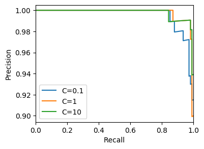
Here we can see the PR curves for each of three hyperparameter configurations. But how did this work? Let’s start by visualizing the dependency graph of our new flow:

flow3.render_dag()

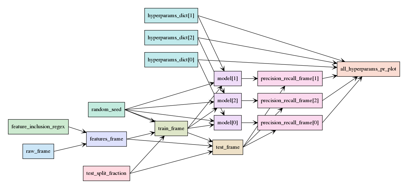
When we specify multiple values for an entity, Bionic creates multiple instances of that entity and of all downstream entities. If there are three instances of hyperparams_dict, there must also be three instances of model and precision_recall_frame.

However, we can also see that there is only one instance of all_hyperparams_plot_pr. This is because we used the @gather decorator when defining this entity: Bionic has aggregated all the variations of hyperparameters_dict and precision_recall_frame into a single frame, so they can be plotted together.

Now, because we have three different model instances, it no longer makes sense to request “the” model:

try:
    flow3.get.model()
except Exception as e:
    caught_exception = e
caught_exception

Loaded      model(feature_inclusion_regex=_.._12aca9f6a2, test_split_fraction=0.3, random_seed=0, hyperparams_dict=ee67dd46dd) from disk cache
Loaded      model(feature_inclusion_regex=_.._12aca9f6a2, test_split_fraction=0.3, random_seed=0, hyperparams_dict=70c34f2de8) from disk cache
Accessed    model(feature_inclusion_regex=_.._12aca9f6a2, test_split_fraction=0.3, random_seed=0, hyperparams_dict=de978d097e) from in-memory cache

ValueError("Entity 'model' has multiple values")

If we want to access an entity with multiple values, we need to tell Bionic what data structure to use to aggregate them:

flow3.get.model('series')

Accessed    model(feature_inclusion_regex=_.._12aca9f6a2, test_split_fraction=0.3, random_seed=0, hyperparams_dict=ee67dd46dd) from in-memory cache
Accessed    model(feature_inclusion_regex=_.._12aca9f6a2, test_split_fraction=0.3, random_seed=0, hyperparams_dict=70c34f2de8) from in-memory cache
Accessed    model(feature_inclusion_regex=_.._12aca9f6a2, test_split_fraction=0.3, random_seed=0, hyperparams_dict=de978d097e) from in-memory cache

feature_inclusion_regex  hyperparams_dict  random_seed  test_split_fraction
W(.*)                    W({'C': 0.1})     W(0)         W(0.3)                 LogisticRegression(C=0.1, class_weight=None, d...
                         W({'C': 1})       W(0)         W(0.3)                 LogisticRegression(C=1, class_weight=None, dua...
                         W({'C': 10})      W(0)         W(0.3)                 LogisticRegression(C=10, class_weight=None, du...
Name: model, dtype: object

Extended Multiplicity

We can apply the same approach to any number of entities:

flow6 = flow3.setting('feature_inclusion_regex', values=['.*', 'mean.*'])
flow6.render_dag()

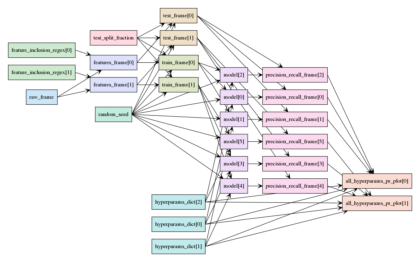
Here we can see that each entity’s multiplicity is propagated through the entire graph. For example, there are two train_frame nodes and two test_frame nodes, because those depend on feature_inclusion_regex but not on hyperparams_dict. However, there are six model nodes, because there are six (two times three) combinations of train_frame and hyperparams_dict.

We can also see two instances of all_hyperparams_pr_plot, corresponding to the two instances of feature_inclusion_regex. This illustrates another nuance of how we used @gather: we asked Bionic to include every variation of hyperparams_dict, along with the associated values of precision_recall_frame. If we had used

@gather(
    over=['hyperparams_dict', 'feature_inclusion_regex'],
    also='precision_recall_frame',
    into='gathered_frame')
def all_variations_pr_plot(...):
    ...

then all the values would be gathered into a single frame, and there would be one single plot node.

Wrapping Up

This tutorial has illustrated four topics:

1. How to use Bionic to assemble a more complex data science flow.

2. How Bionic uses caching to avoid redundant computation.

3. How to repurpose an existing flow to use new parameters or data.

4. How to use multiplicity to compare several variations within a single flow.

These concepts should be enough to get started building real flows. The next section of the documentation will discuss the underlying concepts in Bionic.